|
OmniSketch
0.1
Oh my sketch!
|


|
|
OmniSketch
0.1
Oh my sketch!
|
|
Now that we have installed OmniSketch on your local machine, we are already in a working state to build up new sketches. But before we actually begin to look at or write code in OmniSketch, a few core concepts, along with a typical workflow, should be explained in a bit nuts and bolts.
Flow is the minimal unit that we measure in the streaming scenario. Each packet transmitted in the network, no matter what it layer-2 procotol is or how many bits it have, belongs to a unique flow. Each flow marks one specific connection between a client and a server, so it always lasts for some time and its liveness is manifested by nothing but a series of packets that shift between the source and destination. The reason why we are only interested in measuring a flow, instead of any packets alone, should now be clear: The long-term QoS (Quality of Service) is what we ultimately care about.
The definition of a flow, as you may have expected, is quite flexible. Depending on the usage, one defines a flow by a set of fields in headers at various layers. For example, if you are to detect the status of a Internet host, you may just group all packets emanating from that host into a single flow. I.e., the flow is given by a 1-tuple \(\langle \textrm{src IP}\rangle\). But to achieve a finer granularity on latency per host pair, one may choose a 2-tuple \(\langle \textrm{src IP}, \textrm{dst IP}\rangle\) as the identification of a flow. But this is not the end. Since the transport layer protocol can indeed impact the user exprience of a flow by introducing congestion control mechanism or being endowed with a level of priority when its packets are queued, sometimes one takes a 5-tuple definition \(\langle \textrm{src IP}, \textrm{dst IP}, \textrm{src port}, \textrm{dst port}, \textrm{layer-4 protocol}\rangle\).
All the three versions of definition aforementioned are supported in OmniSketch. The use of these definitions are so prevalent in practice that OmniSketch currently only considers to support these three. You are highly likely to be content with what we have offered so far, but in case that you face inconvenience, please do inform us via email or github. For clarity, we summarize the definition of a flow as follows:
| Definition | Length of the Identification |
|---|---|
| \(\langle \textrm{src IP}\rangle\) | 4 |
| \(\langle \textrm{src IP}, \textrm{dst IP}\rangle\) | 8 (4+4) |
| \(\langle \textrm{src IP}, \textrm{dst IP}, \textrm{src port}, \textrm{dst port}, \textrm{layer-4 protocol}\rangle\) | 13 (4+4+2+2+1) |
Flow, from a different angle, is also what separates the data and the algorithm. Be aware that the raw .pcap or .pcapng file is not usable with OmniSketch, since such file (usually generated by tools like Wireshark or tcpdump) is typically large and contains so many uninterested content such as the application layer payload and pcap-specific packet records. So we add an additional model here, which is properly named as PcapParser, that can be customized to consume a capture file and output in a binary format a succinct file comprised of only packet length, timestamp and flow key information. Any point since OmniSketch is running, all it knows comes from that binary file.
We will not digress to the usage of PcapParser right now. Desultory readers may just skip to read the part on PcapParser.
From what we care about the flow comes the notion of metrics. Metrics are exactly what we want to get out of sketch algorithm eventually. Collecting information per packet is formidable given the line rate and link bandwidth, and is also less intuitive since otherwise, there were going to be too many data! The purpose of a sketch is to provide a summary of the flow-wise statistics, such as flow size (i.e., the number of bytes in the flow), heavy hitters and so on, using only a severely restricted amount of space. Accuracy must be compromised to a pre-agreed \(1-\epsilon\) rather than \(100\%\) in compliance with the fundamental theorem of the information theory.
Good news is that the metrics we are looking for can be categorized into only a handful of types, and the process of collecting these metrics on various sketches are all alike. This drives development of the auto-testing framework of OmniSketch: Users invoke testing routines in a way they want their sketch to be tested, and each test routine collects a subset of all available metrics inside. User can instruct which metrics to include and display by fiddling with the sketch configurations.
Here is a complete list of all available metrics in OmniSketch. Again, if you find your interested metric is not included, please contact us via email or github. We would appreciate your feedback.
| Metric | Description |
|---|---|
SIZE | size (in bytes) of the sketch |
TIME | running time (in microseconds, 1e-6s) of the sketch on a test routine |
RATE | processing rate (packets per second) |
ARE | average relative error |
AAE | average absolute error |
ACC | correct rate |
TP | true positive rate |
FP | false positive rate |
TN | true negative rate |
FN | false negative rate |
PRC | precision rate |
RCL | recall rate |
F1 | harmonic mean of precision & recall (F-one, not F-ell) |
DIST | distribution of the error |
PODF | portion of the desired flow (i.e., whose error is below a threshold) |
RATIO | decoded ratio (in percentile), i.e., the ratio of #(decoded flows) in ground truth to #flows |
Glad you have finished reading main body of the overview! Now it is the time that we summarize a bit and look into the workflow.
The general workflow is nicely depicted in the following.
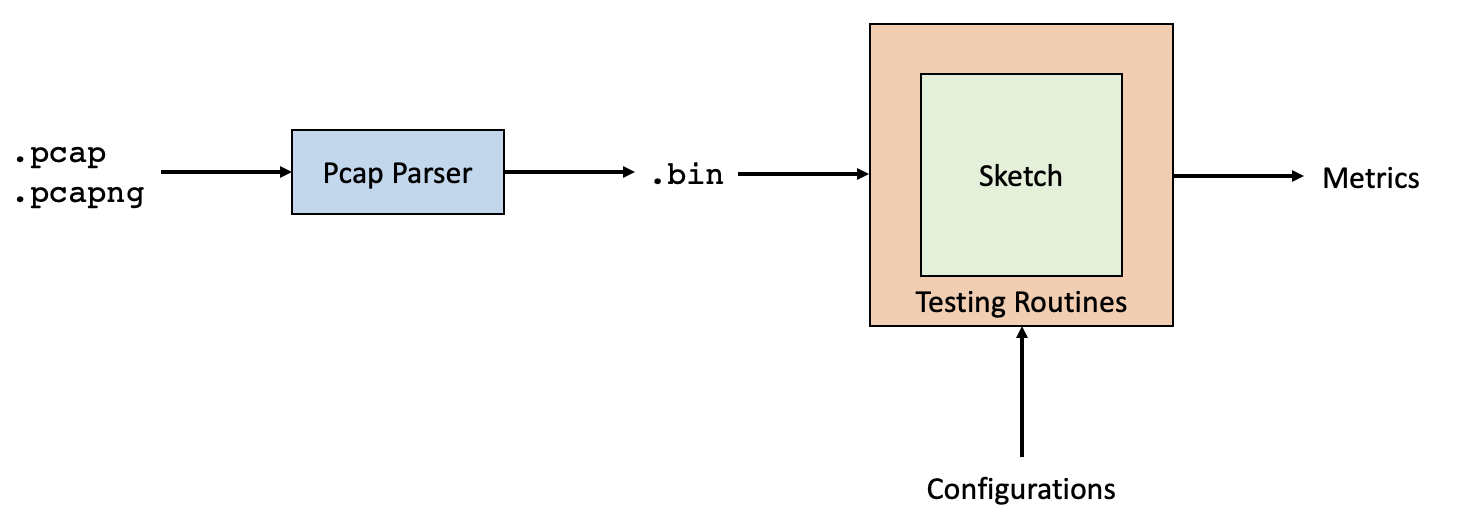
We have learnt that once a capture file goes through Pcap Parser, it contains only flowkey-associated information. Testing routines run atop the sketch algorithm, read the configurations and output metrics that quantitatively measures the goodness of a sketch.
 1.8.17